Big Data Analytics - Data Visualization
In order to understand data, it is often useful to visualize it. Normally in Big Data applications, the interest relies in finding insight rather than just making beautiful plots. The following are examples of different approaches to understanding data using plots.
To start analyzing the flights data, we can start by checking if there are correlations between numeric variables. This code is also available in bda/part1/data_visualization/data_visualization.R file.
# Install the package corrplot by running
install.packages('corrplot')

# then load the library
library(corrplot)

# Load the following libraries
library(nycflights13)
library(ggplot2)
library(data.table)
library(reshape2)

# We will continue working with the flights data
DT <- as.data.table(flights)
head(DT) # take a look

# We select the numeric variables after inspecting the first rows.
numeric_variables = c('dep_time', 'dep_delay',
   'arr_time', 'arr_delay', 'air_time', 'distance')

# Select numeric variables from the DT data.table
dt_num = DT[, numeric_variables, with = FALSE]

# Compute the correlation matrix of dt_num
cor_mat = cor(dt_num, use = "complete.obs")

print(cor_mat)
### Here is the correlation matrix
#              dep_time   dep_delay   arr_time   arr_delay    air_time    distance
# dep_time   1.00000000  0.25961272 0.66250900  0.23230573 -0.01461948 -0.01413373
# dep_delay  0.25961272  1.00000000 0.02942101  0.91480276 -0.02240508 -0.02168090
# arr_time   0.66250900  0.02942101 1.00000000  0.02448214  0.05429603  0.04718917
# arr_delay  0.23230573  0.91480276 0.02448214  1.00000000 -0.03529709 -0.06186776
# air_time  -0.01461948 -0.02240508 0.05429603 -0.03529709  1.00000000  0.99064965
# distance  -0.01413373 -0.02168090 0.04718917 -0.06186776  0.99064965  1.00000000

# We can display it visually to get a better understanding of the data
corrplot.mixed(cor_mat, lower = "circle", upper = "ellipse")

# save it to disk
png('corrplot.png')
print(corrplot.mixed(cor_mat, lower = "circle", upper = "ellipse"))
dev.off()
This code generates the following correlation matrix visualization −
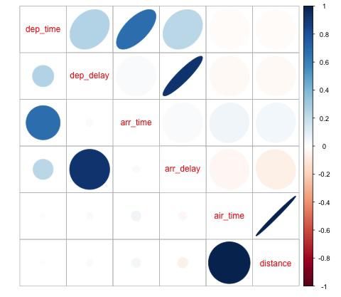
We can see in the plot that there is a strong correlation between some of the variables in the dataset. For example, arrival delay and departure delay seem to be highly correlated. We can see this because the ellipse shows an almost lineal relationship between both variables, however, it is not simple to find causation from this result.
We can’t say that as two variables are correlated, that one has an effect on the other. Also we find in the plot a strong correlation between air time and distance, which is fairly reasonable to expect as with more distance, the flight time should grow.
We can also do univariate analysis of the data. A simple and effective way to visualize distributions are box-plots. The following code demonstrates how to produce box-plots and trellis charts using the ggplot2 library. This code is also available in bda/part1/data_visualization/boxplots.R file.
source('data_visualization.R')
### Analyzing Distributions using box-plots
# The following shows the distance as a function of the carrier

p = ggplot(DT, aes(x = carrier, y = distance, fill = carrier)) + # Define the carrier
   in the x axis and distance in the y axis
   geom_box-plot() + # Use the box-plot geom
   theme_bw() + # Leave a white background - More in line with tufte's
      principles than the default
   guides(fill = FALSE) + # Remove legend
   labs(list(title = 'Distance as a function of carrier', # Add labels
      x = 'Carrier', y = 'Distance'))
p
# Save to disk
png(‘boxplot_carrier.png’)
print(p)
dev.off()

# Let's add now another variable, the month of each flight
# We will be using facet_wrap for this
p = ggplot(DT, aes(carrier, distance, fill = carrier)) +
   geom_box-plot() +
   theme_bw() +
   guides(fill = FALSE) +
   facet_wrap(~month) + # This creates the trellis plot with the by month variable
   labs(list(title = 'Distance as a function of carrier by month',
      x = 'Carrier', y = 'Distance'))
p
# The plot shows there aren't clear differences between distance in different months

# Save to disk
png('boxplot_carrier_by_month.png')
print(p)
dev.off()